Chapter 4 Data Wrangling
Data wrangling is the process of cleaning data, so that data become ready for further manipulation such as visualization and modeling. Sometimes, data wrangling is also called Data Munging. More specifically, data wrangling involves transforming and mapping data from one from to another form - particularly from raw form to tidy form.
There is an old saying that 90% of data science involves data wrangling. In many cases, data wrangling is difficult as it involves dealing with missing entries, ambiguous values, and different types of mixed data. In data analytics ecosystem in R, data wrangling involves three jobs - importing data into R, cleaning (tidying) the data, and transforming the data. Please see Figure 4.1 to learn about the data wrangling process.
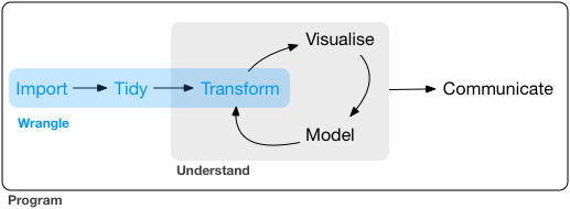
FIGURE4.1: Data Wrangling in R
The first job - importing data into R - is discussed in chapter 03. In this chapter, cleaning (tidying) the data in R will be discussed. The last job will be discussed in next chapter - Exploratory Data Analysis (EDA).
4.1 tidy data
Data wrangling or data munging results in tidy data - which is storing data that makes further manipulation on data such as transformation, visualization, and modeling easier. The following rules make a dataset tidy -
- Each variable must have its own column
- Each observation must have its own row
- Each value must have its own cell
4.2 Same Data, but Different Formats (Presentations)
4.3 Tidying Messy Data
According to Hadley Wickham, “Tidy datasets are all alike, but every messy dataset is messy in its own way” (Wickham and Grolemund 2017). Messy data can be in many forms; for example - Wickham (2014) mentions the five most common problems with messy datasets. These problems include -
- Column headers are values, not variable names
- Multiple variables are stored in one column
- Variables are stored in both rows and columns
- Multiple types of observational units are stored in the same table
- A single observational unit is stored in multiple tables
4.3.1 Column Hearders are Values, not Variable Names
The following dataset (total_assets) is an example of this case, in which the name of the variables (columns) are numbers. Though in some cases, this data format might be useful, in many cases usually it is not useful.
total_assets## # A tibble: 5 x 7
## TICKER COMPANYNAME `2000` `2001` `2002` `2003` `2004`
## <chr> <chr> <dbl> <dbl> <dbl> <dbl> <dbl>
## 1 AAPL APPLE INC 6803 6021 6298 6815 8.05e3
## 2 WMT WALMART INC 70349 78130 83451 94685 1.05e5
## 3 AABA ALTABA INC 2270. 2379. 2790. 5932. 9.18e3
## 4 AMZN AMAZON.COM~ 2135. 1638. 1990. 2162. 3.25e3
## 5 GOOGL ALPHABET I~ NA NA 287. 871. 3.31e34.3.2 Multiple Variables are Stored in One Column
The netincome_asset dataset is a good example of this kind of dataset. For example, the variable VALUES includes net income and total assets separated by /. This variable is very hard to manipulate. For example, if we want to calculate Return on Assets (ROA), which equals to net income divided by total assets, then it is not possible to use VALUES column to calculate ROA.
netincome_asset## # A tibble: 23 x 4
## year TICKER COMPANYNAME VALUES
## <dbl> <chr> <chr> <chr>
## 1 2000 AAPL APPLE INC 786/6803
## 2 2001 AAPL APPLE INC -25/6021
## 3 2002 AAPL APPLE INC 65/6298
## 4 2003 AAPL APPLE INC 69/6815
## 5 2004 AAPL APPLE INC 276/8050
## 6 2000 WMT WALMART INC 5377/70349
## 7 2001 WMT WALMART INC 6295/78130
## 8 2002 WMT WALMART INC 6671/83451
## 9 2003 WMT WALMART INC 8039/94685
## 10 2004 WMT WALMART INC 9054/104912
## # ... with 13 more rows4.3.3 Variables are Stored in Both Rows and Columns
The sales_profit dataset is an example of this type. Here in the ITEM column, actually variables are included (such as SALES and NETINCOME). Also, the columns such as 2000 through 2004 should be a variable (e.g., year).
sales_profit ## # A tibble: 10 x 8
## TICKER COMPANYNAME ITEM `2000` `2001` `2002`
## <chr> <chr> <chr> <dbl> <dbl> <dbl>
## 1 AAPL APPLE INC SALES 7.98e3 5.36e3 5.74e3
## 2 AAPL APPLE INC NETI~ 7.86e2 -2.50e1 6.50e1
## 3 WMT WALMART INC SALES 1.66e5 1.92e5 2.19e5
## 4 WMT WALMART INC NETI~ 5.38e3 6.30e3 6.67e3
## 5 AABA ALTABA INC SALES 1.11e3 7.17e2 9.53e2
## 6 AABA ALTABA INC NETI~ 7.08e1 -9.28e1 4.28e1
## 7 AMZN AMAZON.COM~ SALES 2.76e3 3.12e3 3.93e3
## 8 AMZN AMAZON.COM~ NETI~ -1.41e3 -5.67e2 -1.49e2
## 9 GOOGL ALPHABET I~ SALES NA NA 4.40e2
## 10 GOOGL ALPHABET I~ NETI~ NA NA 9.97e1
## # ... with 2 more variables: `2003` <dbl>,
## # `2004` <dbl>4.3.4 Multiple Types of Observational Units are Stored in the Same Table
4.3.5
4.4 tidyr Package for tidy Data
The tidyr package is widley used to tidy data in R. Specifically, pivot_longer, pivot_wider, separate, and extract functions are widely used to make a messy data into tidy.
4.4.1 pivot_longer () function
If the total_assets dataset above (Column headers are values, not variable names) is made tidy using pivot_longer function, then it will be look like this (Assuming the name of the dataset is variable_number) -
# using pivot_longer () function
total_assets %>%
  pivot_longer(cols = -c("TICKER", "COMPANYNAME"),
               names_to = "year",
               values_to = "TOTALASSETS"
               ) %>%
  head()
## # A tibble: 6 x 4
## TICKER COMPANYNAME year TOTALASSETS
## <chr> <chr> <chr> <dbl>
## 1 AAPL APPLE INC 2000 6803
## 2 AAPL APPLE INC 2001 6021
## 3 AAPL APPLE INC 2002 6298
## 4 AAPL APPLE INC 2003 6815
## 5 AAPL APPLE INC 2004 8050
## 6 WMT WALMART INC 2000 70349There are several arguments of pivot_longer function. Here three arguments are used. The cols argument specifies which columns should (not) be used in pivot_longer function. In this case, we select the variables that should not be used while using pivot_longer function. The second argument names_to specifies the name of the variable in which existing column values will be stored and finally values_to specifies the name of the column in which the cell values will be stored. Now, the dataset is a tidy dataset.
4.4.2 pivot_wider () function
The sales_profit dataset can be put into tidy format using both pivot_longer and pivot_wider function.
sales_profit %>%
  pivot_longer(
    cols = !c ("TICKER", "COMPANYNAME", "ITEM"),
    names_to = "year",
    values_to = "AMOUNT"
  ) %>%
  pivot_wider(
    names_from = ITEM,
    values_from = AMOUNT
  )
## # A tibble: 25 x 5
## TICKER COMPANYNAME year SALES NETINCOME
## <chr> <chr> <chr> <dbl> <dbl>
## 1 AAPL APPLE INC 2000 7983 786
## 2 AAPL APPLE INC 2001 5363 -25
## 3 AAPL APPLE INC 2002 5742 65
## 4 AAPL APPLE INC 2003 6207 69
## 5 AAPL APPLE INC 2004 8279 276
## 6 WMT WALMART INC 2000 165639 5377
## 7 WMT WALMART INC 2001 192003 6295
## 8 WMT WALMART INC 2002 218529 6671
## 9 WMT WALMART INC 2003 245308 8039
## 10 WMT WALMART INC 2004 257157 9054
## # ... with 15 more rows4.4.3 separate () function
The separate function can be used when multiple variables are stored in one column. The function separates one column into multiple columns. For example, in netincome_asset data, the column VALUES should be converted into two columns called NETINCOME and TOTALASSETS. In separate function, col argument is ued to select the column that needs to be broken; into argument is used to create new columns; and sep argument is ued to identify the character in which the column will be separated. In this case, it is /. Finally remove argument is used to decide whether the column (here VALUES) that is separated should be in new dataset.
netincome_asset %>%
  separate(
    col = VALUES, into = c ("NETINCMOE", "TOTALASSETS"), sep ="/",
    remove =TRUE
  )
## # A tibble: 23 x 5
## year TICKER COMPANYNAME NETINCMOE TOTALASSETS
## <dbl> <chr> <chr> <chr> <chr>
## 1 2000 AAPL APPLE INC 786 6803
## 2 2001 AAPL APPLE INC -25 6021
## 3 2002 AAPL APPLE INC 65 6298
## 4 2003 AAPL APPLE INC 69 6815
## 5 2004 AAPL APPLE INC 276 8050
## 6 2000 WMT WALMART INC 5377 70349
## 7 2001 WMT WALMART INC 6295 78130
## 8 2002 WMT WALMART INC 6671 83451
## 9 2003 WMT WALMART INC 8039 94685
## 10 2004 WMT WALMART INC 9054 104912
## # ... with 13 more rowsIt is clear from the above dataset that the type of columns NETINCOME and TOTALASSETS are chr, but they should be number (e.g., dbl). Actually, separate functions maintain the type of the columns that are separated. The type of VALUES column was chr and it is maintained in new dataset. In order to get the true type, we can use convert argument, which is done below.
netincome_asset  %>%
  separate(
    col = VALUES, into = c ("NETINCMOE", "TOTALASSETS"), sep ="/",
    remove =TRUE,convert = TRUE
  )
## # A tibble: 23 x 5
## year TICKER COMPANYNAME NETINCMOE TOTALASSETS
## <dbl> <chr> <chr> <dbl> <dbl>
## 1 2000 AAPL APPLE INC 786 6803
## 2 2001 AAPL APPLE INC -25 6021
## 3 2002 AAPL APPLE INC 65 6298
## 4 2003 AAPL APPLE INC 69 6815
## 5 2004 AAPL APPLE INC 276 8050
## 6 2000 WMT WALMART INC 5377 70349
## 7 2001 WMT WALMART INC 6295 78130
## 8 2002 WMT WALMART INC 6671 83451
## 9 2003 WMT WALMART INC 8039 94685
## 10 2004 WMT WALMART INC 9054 104912
## # ... with 13 more rows4.4.4 extract () function
This is a very good source to discuss about data wrangling - https://dsapps-2020.github.io/Class_Slides/
This is the best data wrangling website - https://dcl-wrangle.stanford.edu/
The above link is also best about why EXCEL is not be best for Accounting & Audit Analytics.